機械学習ライブラリ Scikit-learn (サイキット・ラーン) 使用例

Scikit-learnの使用例 (Irisデータセットの分類)

以下に、Irisデータセットを使って、典型的な分類タスクの流れをまとめた使用例を示します。

import numpy as np
import matplotlib.pyplot as plt
from sklearn.datasets import load_iris
from sklearn.model_selection import train_test_split, GridSearchCV
from sklearn.preprocessing import StandardScaler
from sklearn.pipeline import Pipeline
from sklearn.svm import SVC
from sklearn.metrics import accuracy_score, classification_report, confusion_matrix
import seaborn as sns

# 1. データセットの読み込み
iris = load_iris()
X = iris.data
y = iris.target
target_names = iris.target_names

print("Dataset shape (features, target):", X.shape, y.shape)
print("Target names:", target_names)

# 2. 訓練データとテストデータに分割
X_train, X_test, y_train, y_test = train_test_split(X, y, test_size=0.3, random_state=42, stratify=y)
# stratify=y を指定することで、各クラスの比率を訓練セットとテストセットで維持します。
print("\nTrain set shape:", X_train.shape, y_train.shape)
print("Test set shape:", X_test.shape, y_test.shape)

# 3. パイプラインの構築 (前処理 + モデル)
# 今回はSVM (Support Vector Machine) を使用
pipeline = Pipeline([
    ('scaler', StandardScaler()), # データを標準化
    ('svm', SVC(random_state=42)) # SVMモデル
])

# 4. ハイパーパラメータチューニングのためのグリッドサーチ
# SVMのハイパーパラメータ (Cとgamma) の候補を定義
param_grid = {
    'svm__C': [0.1, 1, 10, 100],
    'svm__gamma': [0.001, 0.01, 0.1, 1]
}

# GridSearchCVのインスタンス化
grid_search = GridSearchCV(pipeline, param_grid, cv=5, scoring='accuracy', n_jobs=-1, verbose=1)
# cv=5: 5分割交差検定
# scoring='accuracy': 評価指標は正解率
# n_jobs=-1: 利用可能なすべてのCPUコアを使用
# verbose=1: ログメッセージを表示

print("\nStarting GridSearchCV...")
grid_search.fit(X_train, y_train)

# 5. 最適なモデルと評価
print("\nBest parameters found by GridSearchCV:")
print(grid_search.best_params_)
print("Best cross-validation accuracy:", grid_search.best_score_)

# 最適なモデルを取得
best_model = grid_search.best_estimator_

# テストデータでの予測
y_pred = best_model.predict(X_test)

# 6. モデルの性能評価
accuracy = accuracy_score(y_test, y_pred)
print(f"\nTest set accuracy: {accuracy:.4f}")

print("\nClassification Report:")
print(classification_report(y_test, y_pred, target_names=target_names))

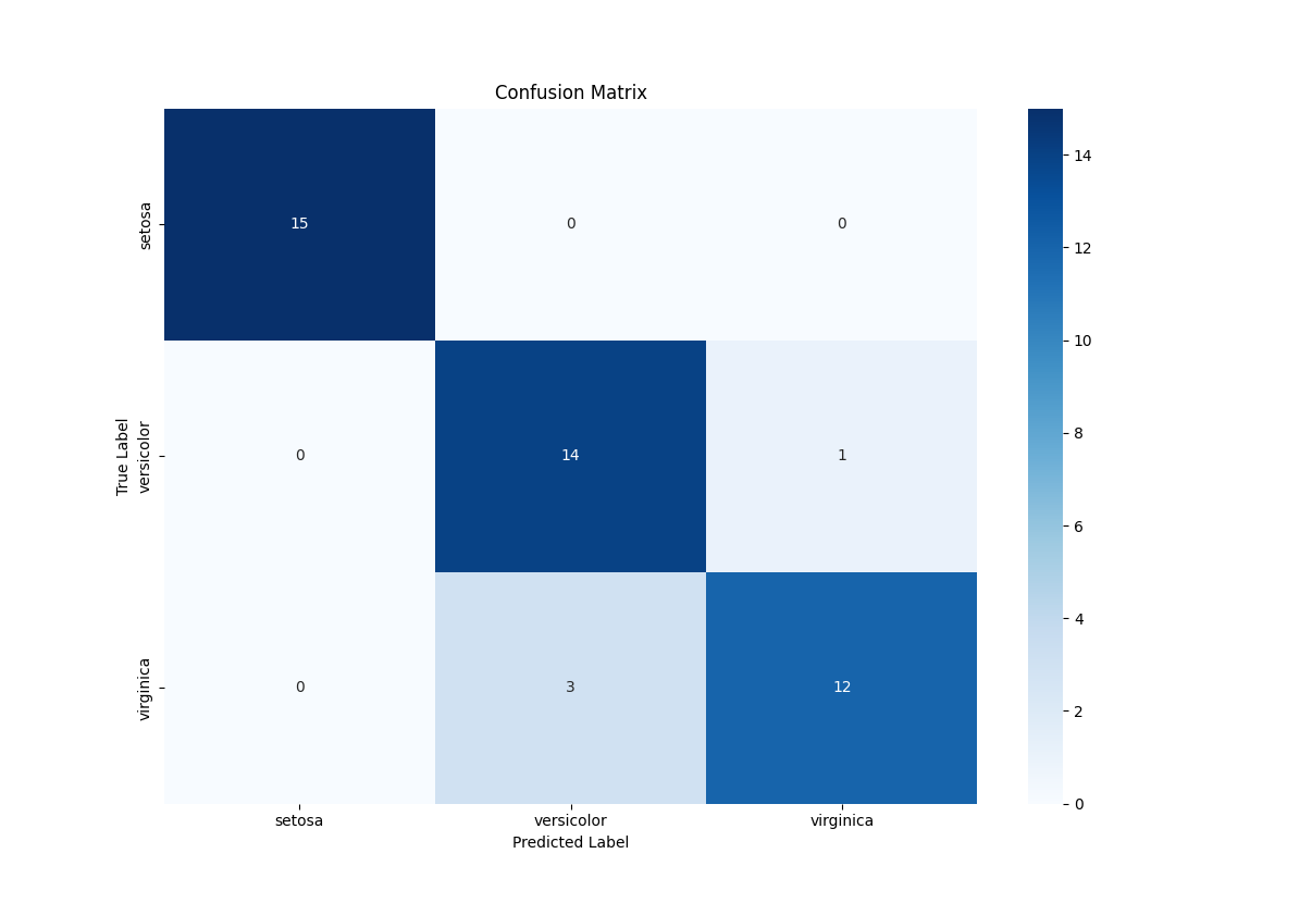
print("\nConfusion Matrix:")
cm = confusion_matrix(y_test, y_pred)
print(cm)

# 混同行列の可視化
plt.figure(figsize=(8, 6))
sns.heatmap(cm, annot=True, fmt='d', cmap='Blues', xticklabels=target_names, yticklabels=target_names)
plt.xlabel('Predicted Label')
plt.ylabel('True Label')
plt.title('Confusion Matrix')
plt.show()

# 7. (オプション) 決定境界の可視化 (2次元に削減してプロット)
# 簡単のために最初の2つの特徴量のみを使用
# データの次元が多い場合、可視化は難しい
from sklearn.decomposition import PCA

if X.shape[1] > 2:
    pca = PCA(n_components=2)
    X_reduced = pca.fit_transform(X)
    X_train_reduced, X_test_reduced, y_train, y_test = train_test_split(X_reduced, y, test_size=0.3, random_state=42, stratify=y)
else:
    X_train_reduced, X_test_reduced = X_train, X_test

# 2次元データでモデルを再学習 (可視化用)
# スケーリングも考慮したパイプライン
plot_pipeline = Pipeline([
    ('scaler', StandardScaler()),
    ('svm', SVC(C=best_model.named_steps['svm'].C, gamma=best_model.named_steps['svm'].gamma, random_state=42))
])
plot_pipeline.fit(X_train_reduced, y_train)

# 決定境界のプロット
x_min, x_max = X_reduced[:, 0].min() - 1, X_reduced[:, 0].max() + 1
y_min, y_max = X_reduced[:, 1].min() - 1, X_reduced[:, 1].max() + 1
xx, yy = np.meshgrid(np.arange(x_min, x_max, 0.02),
                     np.arange(y_min, y_max, 0.02))

Z = plot_pipeline.predict(np.c_[xx.ravel(), yy.ravel()])
Z = Z.reshape(xx.shape)

plt.figure(figsize=(10, 7))
plt.contourf(xx, yy, Z, alpha=0.8, cmap=plt.cm.RdYlBu)
plt.scatter(X_train_reduced[:, 0], X_train_reduced[:, 1], c=y_train, cmap=plt.cm.RdYlBu, edgecolors='k', s=80, label='Train data')
plt.scatter(X_test_reduced[:, 0], X_test_reduced[:, 1], c=y_test, cmap=plt.cm.RdYlBu, edgecolors='k', marker='*', s=100, label='Test data')
plt.xlabel('Principal Component 1')
plt.ylabel('Principal Component 2')
plt.title('SVM Decision Boundary on PCA-reduced Iris Data')
plt.legend()
plt.show()

結果

output_report

この例では、以下のステップを踏んでいます。

データセットの読み込み: Scikit-learnに組み込まれているIrisデータセットを使用します。
データ分割: 訓練データとテストデータに分割し、モデルの汎化性能を評価できるようにします。stratify=yでクラスの偏りを防ぎます。
パイプラインの構築: 前処理（StandardScalerによる標準化）とモデル（SVC）をパイプラインで連結します。これにより、前処理を含めてモデル全体を単一のオブジェクトとして扱えます。
ハイパーパラメータチューニング: GridSearchCVを使って、SVCの最適なハイパーパラメータ(Cとgamma)を探索します。交差検定を用いて過学習を防ぎながら、最適な組み合わせを見つけます。
モデル評価: 最適なモデルを使ってテストデータに対する予測を行い、accuracy_score、classification_report、confusion_matrixでモデルの性能を詳細に評価します。
可視化: 混同行列をヒートマップで表示し、分類結果を視覚的に把握します。また、2次元に削減したデータでの決定境界の可視化も行います。

Scikit-learnは非常に強力で汎用性の高いライブラリであり、これらの基本的な概念とコマンドを理解することで、様々な機械学習タスクに応用することができます。